写在前面
- 支持向量:两类别距离决策边界最近且相等的点。
- SVM目的:使得两个类别的SV间的距离最小。即最大化Margin间的距离。
- SVM考虑当前样本同时,又考虑到未来可能出现的样本,即使找到的决策边界尽量有强的泛化能力。
- 经过数学推到,可以将问题转化为最优化问题。如同其他参数学习算法。
- 其他机器学习算法一般是全局最优化问题,而SVM是有条件的最优化问题。
- 有条件的最优化问题使用拉格朗日算子求解。
- KKT条件
- Hard Margin要严格满足两个Margin见没有没有任何样本点。这由该最优化问题的条件决定。
- Soft Margin允许两个Margin之间存在样本点,即有容错的能力。相应的模型条件与目标都会体现该容错能力。
- L1正则;L2正则
- Hinge损失函数,Exponential Loss,Logistic Loss,是常用的损失函数,由好的数学性质。
- 惩罚项表达了容错空间,不能太大。
- 目标表达式中的
C,目的是平衡前后两部分的比例。 - 此处C(正则化惩罚系数)与其他ML算法C含义不同,但是可以相同地解读。且C越大,越接近Hard Margin。
- SVM中涉及距离,所以要对数据进行标准化处理。否则当不同维数的特征尺度不同时,影响模型性能。
1. 数据
有二分类样本:
1 | iris = datasets.load_iris() |
2. 首先标准化处理:
1 | from sklearn.preprocessing import StandardScaler |
得到标准化后的x_standard。
为了说明问题,使用所有数据fit,使用原来数据predict。
3. 当C取很大值时,如C=1e9:
1 | svc = LinearSVC(C=1e9) |
查看模型所学,w和b:
1 | print(svc.coef_) # w [[ 4.03242779 -2.49296705]] |
绘出决策边界, 及两个Margin:
1 | plot_svc_decision_boundary(svc, axis=[-3, 3, -3, 3]) |
如图:
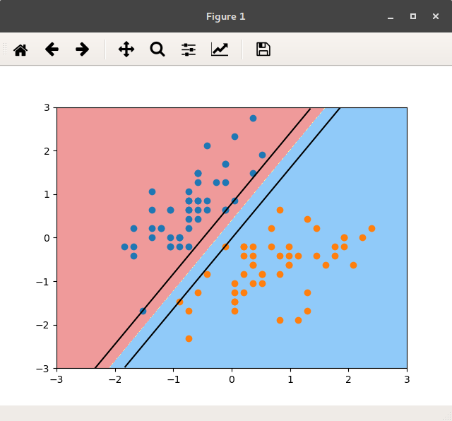
图 C=1e9的分类边界
4. 当C取很小值时,如C=0.05:
1 | svc2 = LinearSVC(C=0.005) |
查看模型所学,w&b:
1 | print(svc2.coef_) # w [[ 0.33360588 -0.30904355]] |
绘出决策边界,及两个Margin:
1 | plot_svc_decision_boundary(svc2, axis=[-3, 3, -3, 3]) |
如图:
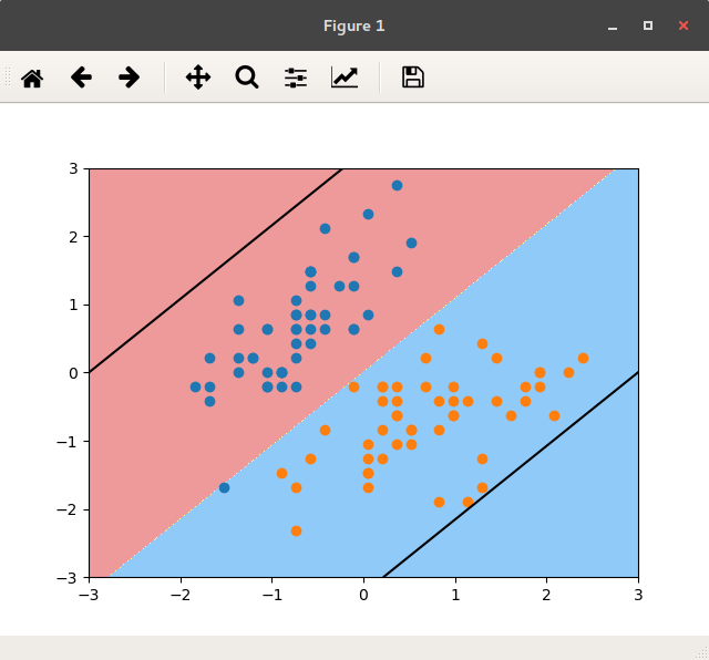
图 C=0.005的分类边界
当C太小时,容错空间太大,以至于大量明显分错的点也被模型认为是允许的。
这是当只指明C后,模型的参数:
1 | LinearSVC(C=1000000000.0, class_weight=None, dual=True, f it_intercept=True, |
可以看出,使用的是hinge损失函数,L2正则化,ovr…等其他设置。
附件
绘出决策边界,及两个Margin的函数:
1 | # show margins and boundary: |